实战:使用 ElasticSearch 8.13 实现混合搜索(4):使用开源模型,导入真实世界数据

2024-04-29 09:19:51 -0400

从本文开始我们终于要开始使用 Python 了,数据量实在超越了 Kibana 控制台能处理的规模。 文末会附带 Jupyter Notebook 示例代码,以保证实验的可复现性。

使用开源模型

Cohere 不是免费的,如果把我们的 50 万条数据都丢给 Cohere embedding 算法处理的话,恐怕要产生一笔我们并不想要的信用卡债。 这一步骤事实上已经在 ElasticSearch 官网博客提供的指南 及其示例代码 Jupyter Notebook 中提及。 测试中发现的易出 bug 点在于 eland[pytorch] 库需要 Python 3.10 才能较为顺利的安装。

这里还有一个问题,我们部署本地开源模型的话,需要使用 GPU 加速的云服务,这笔信用卡债似乎很难躲开。 但如果我们的数据规模扩张到难以控制的程度,这笔实践经验就会显得十分宝贵。 我们使用 AWS 最便宜的 g4dn.xlarge 实例运行我们的 PyTorch 服务。 虽然他提供的 nVidia T4 GPU 已经是五年前发布的,但是 T4 GPU 似乎为半精度浮点计算( FP16 )做了特殊的优化,其半精度浮点计算能力高达 65.13 TFLOPS ,十分符合我们的需求。

当然,云服务价格比 r7gd.large 贵了四倍。 而且需要从 AWS 申请限额,可能要等一天才能完成。 我们先在本机上玩,玩透了大概 AWS 也批准了我们的限额请求了。

笔者笔电的 RTX 2070 Max-Q 在大概 4 秒钟之内完成了 Cohere embedding 需要一分钟, CPU 十分钟不一定跑的完的数据,赢麻了。

另外还有一个容易卡住的点,可以参考这一节

更新: AWS 拒绝了我们提高服务限额的申请。 但工程领域总有绕过的手段,既然我们并不追求数据的实时更新,我们可以先在我们的笔电上完成数据的索引,再通过 elasticsearch-dump 上传到云服务上,这不就赢麻了嘛。

使用 Celery / RabbitMQ 管理大规模数据操作

笔者简单尝试了一下使用 Python 和 ElasticSearch 自带的 bulk 工具导入 50 万条评论数据,效果不佳,事实上仅仅导入了 10 万条。

输入 Best pasta in New York 执行搜索,搜索结果的确令人满意

ID: 32390
Doc Title: review_720045084
Restaurant Name: Tony_s_Di_Napoli_Midtown
Title Review: Fantastic food!
Passage Text:
The best pasta in New York! Great dessert and friendly staff. A bit noisy on a Sunday evening but a really nice evening close to Times square.

Score: 0.9367155
---
ID: 52686
Doc Title: review_651849097
Restaurant Name: Carmine_s_Italian_Restaurant_Times_Square
Title Review: Wonderful
Passage Text:
The best pasta in New York. The only problem is the size of the plates. They must do smaller plates. For one person for example.

Score: 0.90883017
---
ID: 73133
Doc Title: review_628690226
Restaurant Name: Il_Gattopardo
Title Review: Excellence
Passage Text:
Perhaps the best pasta in NY. They can deliver pasta al dente, as they have done that for us in the past.

Score: 0.89915013
---
ID: 1460
Doc Title: review_609031069
Restaurant Name: San_Carlo_Osteria_Piemonte
Title Review: Good if you are not italian
Passage Text:
Nice food in New York if you are not Italian but if you know how Italian food really is you can cook better at your home.Pasta not good

Score: 0.88570404
---
ID: 149
Doc Title: review_695311754
Restaurant Name: San_Carlo_Osteria_Piemonte
Title Review: Outstanding food,  great service and atmosphere 
Passage Text:
I'm a huge fan of picolla cucina on Spring St and I still think they have the best pastas in New York. It's my favorite in NYC, but a block away is San Carlo which may bemy second favorite. It is slightly different in terms of the menu, with less focus on pasta. It also has a slightly larger footprint with a small intimate bar, and has a very good wine and cocktail list.

Score: 0.8833201
---
ID: 70098
Doc Title: review_417272677
Restaurant Name: Forlini_s_Restaurant
Title Review: Buenísimo!!!
Passage Text:
Best pasta and minestrone soup ever, we been looking around in little Italy New york for a good Italian restaurant, I consult trip advisor. Found the place and was a delightful surprise. Jack where our hostess very kind and funny man. Definitely we are going to come back soon during our trip here in NY.

Score: 0.8831816
---
ID: 87324
Doc Title: review_241290115
Restaurant Name: Carmine_s_Italian_Restaurant_Times_Square
Title Review: Real Italian food
Passage Text:
Best classic Italian food in NYC.

Score: 0.8803612
---
ID: 21092
Doc Title: review_629514788
Restaurant Name: IL_Melograno
Title Review: Tastefull meal - worth a visit!!
Passage Text:
Best meal we’ve had in NYC! The pasta was just delicious / super fresh & the staff very friendly and kind. We would recommend it for sure!

Score: 0.8786392
---
ID: 22079
Doc Title: review_375834633
Restaurant Name: Orso
Title Review: Always a crowd pleaser!
Passage Text:
Love this restaurant and still mourn the closing of the LA spot. The best pastas and a perfect place to have lunch that "feels" like NYC! Very traditional and located very near the theater district, so you can hop in for an early dinner pre-show as well. You really can't go wrong ordering everything on the menu but my last visit, I had them make me a simple pasta with tomatoes and basil.

Score: 0.8776474
---
ID: 69039
Doc Title: review_467680511
Restaurant Name: Forlini_s_Restaurant
Title Review: The best. The very best.
Passage Text:
If tradition, quality service, and first-rate homemade pasta is your desire, then look no more. This place is simply the best in NYC. I've been here several times after stumbling on it last year. Wish I had found it earlier in my career; it would have made many of my previous visits to NYC even more satisfying to the palate -- and wallet. Love the family atmosphere.

Score: 0.8749021

笔者决定使用大规模分布式数据处理的保留手段, RabbitMQ + Celery + 多个 Celery worker 。 只需要简单编辑一下 docker-compose.yml ,新建 Celery worker 的代码Dockerfile ,即可享受大规模分布式数据处理的乐趣。

实验结果和代码样例

RabbitMQ控制台

根据 RabbitMQ 控制台,我们在大概 30 分钟的时间里完成了 10% 的数据索引,那么索引整个 50 万条 review 大约需要 5 个小时左右。

这里的瓶颈是我们的 docker-compose 自动提供的 ES 集群是单线程的。 为了节约配置的时间,我们在最初进行原型开发的时候可以直接使用 Elastic Cloud 针对推理优化过的集群。

代码样例: Jupyter Notebook

这一代码样例实现了实验计划的全部功能(除 re-ranking 之外):

  1. 语义搜索:验证 Cohere 提供的 embedding 算法和 ElasticSearch 的 ANN 搜索。
  2. 建立 ES 的导入数据 Ingest Pipeline, chunking 长文到合适规模。
  3. 导入真实世界测试数据: TripAdvisor 上的 50 万条纽约市餐厅评论

下文预告

我们在本节中使用 ES 的 ingest pipeline 引入大规模数据,测试语义搜索功能。

下一节将测试 Cohere 提供的 re-ranking 算法,在前 100 条

纽约最好的意大利面饭馆

中,重新排序出第一二三四名来。

实验计划

  1. 小样本测试
    1. 语义搜索:验证 Cohere 提供的 embedding 算法和 ElasticSearch 的 ANN 搜索。
    2. 建立 ES 的导入数据 Ingest Pipeline, chunking 长文到合适规模。
    3. 重排序:验证 Cohere 提供的 re-ranking 算法
  2. 大样本测试:
    1. 构建本地测试环境
    2. 导入真实世界测试数据

本节完成了 2.2 。

实战:使用 ElasticSearch 8.13 实现混合搜索(3):构建长文拆分管线( chunking )

2024-04-29 07:52:59 -0400

长文拆分

与支持无限长文分析的 BM25 技术不同, Cohere 提供的 embedding 算法是不能处理超过 1024 个 token 的文字的。对于长度超过 128 个 token 的文本, Cohere 的算法将会切分其 embedding 结果向量,取其平均值1

根据 ElasticSearch 官网博客提供的指南,我们对 Kibana 控制台输入以下命令。 请注意这里的向量维度被更改为了 1024 维,相似性算法也不再是指南中提供的向量点乘,而是余弦,以适应 Cohere 的 embedding 算法。

PUT chunker
{
  "mappings": {
    "dynamic": "true",
    "properties": {
      "passages": {
        "type": "nested",
        "properties": {
          "vector": {
            "properties": {
              "predicted_value": {
                "type": "dense_vector",
                "index": true,
                "dims": 1024,
                "similarity": "cosine"
              }
            }
          }
        }
      }
    }
  }
}

我们继续,构建 Ingest 管线。 例子中提供的管线包括两个预处理步骤:

  1. 使用正则表达式把 body_content 中的内容切分为一组句子,这里的正则表达式规避了不正确切分的做法(如在 Mr. 或 Mrs. 上切分)。
  2. 尝试把句子块连缀起来,使其尽可能接近我们设定的长度上限。

预处理步骤之后,管线对每个句子执行 embedding 算法。 请注意我们每段文章有若干段文本块( chunk ,在我们的索引中是 passage.text ),每个文本块都有其 embedding 之后的向量,即之前所定义的 passage.vector.predicted_value

PUT _ingest/pipeline/chunker
{
  "processors": [
    {
      "script": {
        "description": "Chunk body_content into sentences by looking for . followed by a space",
        "lang": "painless",
        "source": """
          String[] envSplit = /((?<!M(r|s|rs)\.)(?<=\.) |(?<=\!) |(?<=\?) )/.split(ctx['body_content']);
          ctx['passages'] = new ArrayList();
          int i = 0;
          boolean remaining = true;
          if (envSplit.length == 0) {
            return
          } else if (envSplit.length == 1) {
            Map passage = ['text': envSplit[0]];ctx['passages'].add(passage)
          } else {
            while (remaining) {
              Map passage = ['text': envSplit[i++]];
              while (i < envSplit.length && passage.text.length() + envSplit[i].length() < params.model_limit) {passage.text = passage.text + ' ' + envSplit[i++]}
              if (i == envSplit.length) {remaining = false}
              ctx['passages'].add(passage)
            }
          }
          """,
        "params": {
          "model_limit": 400
        }
      }
    },
    {
      "foreach": {
        "field": "passages",
        "processor": {
          "inference": {
            "model_id": "cohere_embeddings",
            "input_output": [
              { 
                "input_field": "_ingest._value.text",
                "output_field": "_ingest._value.vector.predicted_value"
              }
            ],
            "on_failure": [
              {
                "append": {
                  "field": "_source._ingest.inference_errors",
                  "value": [
                    {
                      "message": "Processor 'inference' in pipeline 'ml-inference-title-vector' failed with message ''",
                      "pipeline": "ml-inference-title-vector",
                      "timestamp": "}"
                    }
                  ]
                }
              }
            ]
          }
        }
      }
    }
  ]
}

插入小样本实验数据:

PUT chunker/_doc/1?pipeline=chunker
{
"title": "Adding passage vector search to Lucene",
"body_content": "Vector search is a powerful tool in the information retrieval tool box. Using vectors alongside lexical search like BM25 is quickly becoming commonplace. But there are still a few pain points within vector search that need to be addressed. A major one is text embedding models and handling larger text input. Where lexical search like BM25 is already designed for long documents, text embedding models are not. All embedding models have limitations on the number of tokens they can embed. So, for longer text input it must be chunked into passages shorter than the model’s limit. Now instead of having one document with all its metadata, you have multiple passages and embeddings. And if you want to preserve your metadata, it must be added to every new document. A way to address this is with Lucene's “join” functionality. This is an integral part of Elasticsearch’s nested field type. It makes it possible to have a top-level document with multiple nested documents, allowing you to search over nested documents and join back against their parent documents. This sounds perfect for multiple passages and vectors belonging to a single top-level document! This is all awesome! But, wait, Elasticsearch® doesn’t support vectors in nested fields. Why not, and what needs to change? The key issue is how Lucene can join back to the parent documents when searching child vector passages. Like with kNN pre-filtering versus post-filtering, when the joining occurs determines the result quality and quantity. If a user searches for the top four nearest parent documents (not passages) to a query vector, they usually expect four documents. But what if they are searching over child vector passages and all four of the nearest vectors are from the same parent document? This would end up returning just one parent document, which would be surprising. This same kind of issue occurs with post-filtering."
}

PUT chunker/_doc/3?pipeline=chunker
{
"title": "Automatic Byte Quantization in Lucene",
"body_content": "While HNSW is a powerful and flexible way to store and search vectors, it does require a significant amount of memory to run quickly. For example, querying 1MM float32 vectors of 768 dimensions requires roughly 1,000,000∗4∗(768+12)=3120000000≈31,000,000∗4∗(768+12)=3120000000bytes≈3GB of ram. Once you start searching a significant number of vectors, this gets expensive. One way to use around 75% less memory is through byte quantization. Lucene and consequently Elasticsearch has supported indexing byte vectors for some time, but building these vectors has been the user's responsibility. This is about to change, as we have introduced int8 scalar quantization in Lucene. All quantization techniques are considered lossy transformations of the raw data. Meaning some information is lost for the sake of space. For an in depth explanation of scalar quantization, see: Scalar Quantization 101. At a high level, scalar quantization is a lossy compression technique. Some simple math gives significant space savings with very little impact on recall. Those used to working with Elasticsearch may be familiar with these concepts already, but here is a quick overview of the distribution of documents for search. Each Elasticsearch index is composed of multiple shards. While each shard can only be assigned to a single node, multiple shards per index gives you compute parallelism across nodes. Each shard is composed as a single Lucene Index. A Lucene index consists of multiple read-only segments. During indexing, documents are buffered and periodically flushed into a read-only segment. When certain conditions are met, these segments can be merged in the background into a larger segment. All of this is configurable and has its own set of complexities. But, when we talk about segments and merging, we are talking about read-only Lucene segments and the automatic periodic merging of these segments. Here is a deeper dive into segment merging and design decisions."
}

PUT chunker/_doc/2?pipeline=chunker
{
"title": "Use a Japanese language NLP model in Elasticsearch to enable semantic searches",
"body_content": "Quickly finding necessary documents from among the large volume of internal documents and product information generated every day is an extremely important task in both work and daily life. However, if there is a high volume of documents to search through, it can be a time-consuming process even for computers to re-read all of the documents in real time and find the target file. That is what led to the appearance of Elasticsearch® and other search engine software. When a search engine is used, search index data is first created so that key search terms included in documents can be used to quickly find those documents. However, even if the user has a general idea of what type of information they are searching for, they may not be able to recall a suitable keyword or they may search for another expression that has the same meaning. Elasticsearch enables synonyms and similar terms to be defined to handle such situations, but in some cases it can be difficult to simply use a correspondence table to convert a search query into a more suitable one. To address this need, Elasticsearch 8.0 released the vector search feature, which searches by the semantic content of a phrase. Alongside that, we also have a blog series on how to use Elasticsearch to perform vector searches and other NLP tasks. However, up through the 8.8 release, it was not able to correctly analyze text in languages other than English. With the 8.9 release, Elastic added functionality for properly analyzing Japanese in text analysis processing. This functionality enables Elasticsearch to perform semantic searches like vector search on Japanese text, as well as natural language processing tasks such as sentiment analysis in Japanese. In this article, we will provide specific step-by-step instructions on how to use these features."
}

PUT chunker/_doc/5?pipeline=chunker
{
"title": "We can chunk whatever we want now basically to the limits of a document ingest",
"body_content": """Chonk is an internet slang term used to describe overweight cats that grew popular in the late summer of 2018 after a photoshopped chart of cat body-fat indexes renamed the "Chonk" scale grew popular on Twitter and Reddit. Additionally, "Oh Lawd He Comin'," the final level of the Chonk Chart, was adopted as an online catchphrase used to describe large objects, animals or people. It is not to be confused with the Saturday Night Live sketch of the same name. The term "Chonk" was popularized in a photoshopped edit of a chart illustrating cat body-fat indexes and the risk of health problems for each class (original chart shown below). The first known post of the "Chonk" photoshop, which classifies each cat to a certain level of "chonk"-ness ranging from "A fine boi" to "OH LAWD HE COMIN," was posted to Facebook group THIS CAT IS C H O N K Y on August 2nd, 2018 by Emilie Chang (shown below). The chart surged in popularity after it was tweeted by @dreamlandtea[1] on August 10th, 2018, gaining over 37,000 retweets and 94,000 likes (shown below). After the chart was posted there, it began growing popular on Reddit. It was reposted to /r/Delighfullychubby[2] on August 13th, 2018, and /r/fatcats on August 16th.[3] Additionally, cats were shared with variations on the phrase "Chonk." In @dreamlandtea's Twitter thread, she rated several cats on the Chonk scale (example, shown below, left). On /r/tumblr, a screenshot of a post featuring a "good luck cat" titled "Lucky Chonk" gained over 27,000 points (shown below, right). The popularity of the phrase led to the creation of a subreddit, /r/chonkers,[4] that gained nearly 400 subscribers in less than a month. Some photoshops of the chonk chart also spread on Reddit. For example, an edit showing various versions of Pikachu on the chart posted to /r/me_irl gained over 1,200 points (shown below, left). The chart gained further popularity when it was posted to /r/pics[5] September 29th, 2018."""
}

如果对 embedding 之后的结果不太放心,我们可以手动观察一下:

GET chunker/_search?size=5
{
    "query": {
        "match_all": {}
    }
}

搜索测试

我们先用官方文档中测试一下,当然 kNN 的搜索 k 不一定一定是 1 ,我们改成 2 。

GET chunker/_search
{
  "_source": false,
  "fields": [
    "title"
  ],
  "knn": {
    "inner_hits": {
      "_source": false,
      "fields": [
        "passages.text"
      ]
    },
    "field": "passages.vector.predicted_value",
    "k": 2,
    "num_candidates": 100,
    "query_vector_builder": {
      "text_embedding": {
        "model_id": "cohere_embeddings",
        "model_text": "Can I use multiple vectors per document now?"
      }
    }
  }
}

搜索结果:

{
  "took": 285,
  "timed_out": false,
  "_shards": {
    "total": 1,
    "successful": 1,
    "skipped": 0,
    "failed": 0
  },
  "hits": {
    "total": {
      "value": 2,
      "relation": "eq"
    },
    "max_score": 0.78212404,
    "hits": [
      {
        "_index": "chunker",
        "_id": "1",
        "_score": 0.78212404,
        "_ignored": [
          "body_content.keyword",
          "passages.text.keyword"
        ],
        "fields": {
          "title": [
            "Adding passage vector search to Lucene"
          ]
        },
        "inner_hits": {
          "passages": {
            "hits": {
              "total": {
                "value": 6,
                "relation": "eq"
              },
              "max_score": 0.78212404,
              "hits": [
                {
                  "_index": "chunker",
                  "_id": "1",
                  "_nested": {
                    "field": "passages",
                    "offset": 3
                  },
                  "_score": 0.78212404,
                  "fields": {
                    "passages": [
                      {
                        "text": [
                          "This sounds perfect for multiple passages and vectors belonging to a single top-level document! This is all awesome! But, wait, Elasticsearch® doesn’t support vectors in nested fields. Why not, and what needs to change? The key issue is how Lucene can join back to the parent documents when searching child vector passages."
                        ]
                      }
                    ]
                  }
                },
                {
                  "_index": "chunker",
                  "_id": "1",
                  "_nested": {
                    "field": "passages",
                    "offset": 0
                  },
                  "_score": 0.7376485,
                  "fields": {
                    "passages": [
                      {
                        "text": [
                          "Vector search is a powerful tool in the information retrieval tool box. Using vectors alongside lexical search like BM25 is quickly becoming commonplace. But there are still a few pain points within vector search that need to be addressed. A major one is text embedding models and handling larger text input."
                        ]
                      }
                    ]
                  }
                },
                {
                  "_index": "chunker",
                  "_id": "1",
                  "_nested": {
                    "field": "passages",
                    "offset": 4
                  },
                  "_score": 0.7086177,
                  "fields": {
                    "passages": [
                      {
                        "text": [
                          "Like with kNN pre-filtering versus post-filtering, when the joining occurs determines the result quality and quantity. If a user searches for the top four nearest parent documents (not passages) to a query vector, they usually expect four documents. But what if they are searching over child vector passages and all four of the nearest vectors are from the same parent document?"
                        ]
                      }
                    ]
                  }
                }
              ]
            }
          }
        }
      },
      {
        "_index": "chunker",
        "_id": "2",
        "_score": 0.704564,
        "_ignored": [
          "body_content.keyword",
          "passages.text.keyword"
        ],
        "fields": {
          "title": [
            "Use a Japanese language NLP model in Elasticsearch to enable semantic searches"
          ]
        },
        "inner_hits": {
          "passages": {
            "hits": {
              "total": {
                "value": 6,
                "relation": "eq"
              },
              "max_score": 0.704564,
              "hits": [
                {
                  "_index": "chunker",
                  "_id": "2",
                  "_nested": {
                    "field": "passages",
                    "offset": 3
                  },
                  "_score": 0.704564,
                  "fields": {
                    "passages": [
                      {
                        "text": [
                          "Elasticsearch enables synonyms and similar terms to be defined to handle such situations, but in some cases it can be difficult to simply use a correspondence table to convert a search query into a more suitable one. To address this need, Elasticsearch 8.0 released the vector search feature, which searches by the semantic content of a phrase."
                        ]
                      }
                    ]
                  }
                },
                {
                  "_index": "chunker",
                  "_id": "2",
                  "_nested": {
                    "field": "passages",
                    "offset": 4
                  },
                  "_score": 0.6868271,
                  "fields": {
                    "passages": [
                      {
                        "text": [
                          "Alongside that, we also have a blog series on how to use Elasticsearch to perform vector searches and other NLP tasks. However, up through the 8.8 release, it was not able to correctly analyze text in languages other than English. With the 8.9 release, Elastic added functionality for properly analyzing Japanese in text analysis processing."
                        ]
                      }
                    ]
                  }
                },
                {
                  "_index": "chunker",
                  "_id": "2",
                  "_nested": {
                    "field": "passages",
                    "offset": 0
                  },
                  "_score": 0.6548239,
                  "fields": {
                    "passages": [
                      {
                        "text": [
                          "Quickly finding necessary documents from among the large volume of internal documents and product information generated every day is an extremely important task in both work and daily life. However, if there is a high volume of documents to search through, it can be a time-consuming process even for computers to re-read all of the documents in real time and find the target file."
                        ]
                      }
                    ]
                  }
                }
              ]
            }
          }
        }
      }
    ]
  }
}

可见文档 1 的相关性有 0.78 ,的确远比相关性只有 0.7 的文档 2 更贴近我们的问题。

我们换一个搜索关键字, scalar quantization ,搜索结果如下:

{
  "took": 424,
  "timed_out": false,
  "_shards": {
    "total": 1,
    "successful": 1,
    "skipped": 0,
    "failed": 0
  },
  "hits": {
    "total": {
      "value": 2,
      "relation": "eq"
    },
    "max_score": 0.8421624,
    "hits": [
      {
        "_index": "chunker",
        "_id": "3",
        "_score": 0.8421624,
        "_ignored": [
          "body_content.keyword",
          "passages.text.keyword"
        ],
        "fields": {
          "title": [
            "Automatic Byte Quantization in Lucene"
          ]
        },
        "inner_hits": {
          "passages": {
            "hits": {
              "total": {
                "value": 6,
                "relation": "eq"
              },
              "max_score": 0.8421624,
              "hits": [
                {
                  "_index": "chunker",
                  "_id": "3",
                  "_nested": {
                    "field": "passages",
                    "offset": 2
                  },
                  "_score": 0.8421624,
                  "fields": {
                    "passages": [
                      {
                        "text": [
                          "Meaning some information is lost for the sake of space. For an in depth explanation of scalar quantization, see: Scalar Quantization 101. At a high level, scalar quantization is a lossy compression technique. Some simple math gives significant space savings with very little impact on recall."
                        ]
                      }
                    ]
                  }
                },
                {
                  "_index": "chunker",
                  "_id": "3",
                  "_nested": {
                    "field": "passages",
                    "offset": 1
                  },
                  "_score": 0.7212088,
                  "fields": {
                    "passages": [
                      {
                        "text": [
                          "One way to use around 75% less memory is through byte quantization. Lucene and consequently Elasticsearch has supported indexing byte vectors for some time, but building these vectors has been the user's responsibility. This is about to change, as we have introduced int8 scalar quantization in Lucene. All quantization techniques are considered lossy transformations of the raw data."
                        ]
                      }
                    ]
                  }
                },
                {
                  "_index": "chunker",
                  "_id": "3",
                  "_nested": {
                    "field": "passages",
                    "offset": 0
                  },
                  "_score": 0.62174904,
                  "fields": {
                    "passages": [
                      {
                        "text": [
                          "While HNSW is a powerful and flexible way to store and search vectors, it does require a significant amount of memory to run quickly. For example, querying 1MM float32 vectors of 768 dimensions requires roughly 1,000,000∗4∗(768+12)=3120000000≈31,000,000∗4∗(768+12)=3120000000bytes≈3GB of ram. Once you start searching a significant number of vectors, this gets expensive."
                        ]
                      }
                    ]
                  }
                }
              ]
            }
          }
        }
      },
      {
        "_index": "chunker",
        "_id": "1",
        "_score": 0.60923594,
        "_ignored": [
          "body_content.keyword",
          "passages.text.keyword"
        ],
        "fields": {
          "title": [
            "Adding passage vector search to Lucene"
          ]
        },
        "inner_hits": {
          "passages": {
            "hits": {
              "total": {
                "value": 6,
                "relation": "eq"
              },
              "max_score": 0.60923594,
              "hits": [
                {
                  "_index": "chunker",
                  "_id": "1",
                  "_nested": {
                    "field": "passages",
                    "offset": 3
                  },
                  "_score": 0.60923594,
                  "fields": {
                    "passages": [
                      {
                        "text": [
                          "This sounds perfect for multiple passages and vectors belonging to a single top-level document! This is all awesome! But, wait, Elasticsearch® doesn’t support vectors in nested fields. Why not, and what needs to change? The key issue is how Lucene can join back to the parent documents when searching child vector passages."
                        ]
                      }
                    ]
                  }
                },
                {
                  "_index": "chunker",
                  "_id": "1",
                  "_nested": {
                    "field": "passages",
                    "offset": 0
                  },
                  "_score": 0.59735155,
                  "fields": {
                    "passages": [
                      {
                        "text": [
                          "Vector search is a powerful tool in the information retrieval tool box. Using vectors alongside lexical search like BM25 is quickly becoming commonplace. But there are still a few pain points within vector search that need to be addressed. A major one is text embedding models and handling larger text input."
                        ]
                      }
                    ]
                  }
                },
                {
                  "_index": "chunker",
                  "_id": "1",
                  "_nested": {
                    "field": "passages",
                    "offset": 2
                  },
                  "_score": 0.59269404,
                  "fields": {
                    "passages": [
                      {
                        "text": [
                          "And if you want to preserve your metadata, it must be added to every new document. A way to address this is with Lucene's “join” functionality. This is an integral part of Elasticsearch’s nested field type. It makes it possible to have a top-level document with multiple nested documents, allowing you to search over nested documents and join back against their parent documents."
                        ]
                      }
                    ]
                  }
                }
              ]
            }
          }
        }
      }
    ]
  }
}

这次则是 0.84 对比 0.6 ,相关性差别十分显著。

下文预告

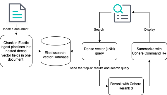
我们在本节中使用了 ES 的 ingest pipeline 引入长文数据,测试了针对长文的语义搜索功能。 工程实现效果是令人满意的。

下文中我们将导入真实世界测试数据,即 Kaggle 上的 Six TripAdvisor Datasets for NLP Tasks2 中的纽约餐厅评论,以验证 ElasticSearch 的 kNN 搜索算法针对大规模数据集的威力。 测试用例暂定为:

找寻纽约最好的意大利面饭馆

实验计划

  1. 小样本测试
    1. 语义搜索:验证 Cohere 提供的 embedding 算法和 ElasticSearch 的 ANN 搜索。
    2. 建立 ES 的导入数据 Ingest 管线, chunking 长文到合适规模。
    3. 重排序:验证 Cohere 提供的 re-ranking 算法
  2. 大样本测试:
    1. 构建本地测试环境
    2. 导入真实世界测试数据

本节实现了 1.2。

实战:使用 ElasticSearch 8.13 实现混合搜索(2):构建本地测试环境

2024-04-27 11:57:19 -0400

构建开发环境: ELK-B

开发环境: AWS EC2 spot instance r7gd.large, ap-southeast-1, Debian 12 (bookworm)

(笔者现在的网络环境不是特别好,用流量下载 docker 镜像实在不太现实)

r7gd.large 有 16 GiB 内存,足够我们搞一搞原型开发。 它提供的 118 GiB NVMe SSD 会在断电后立刻擦除全部数据,可以暂缓对其利用)

我们使用 docker-compose 构建开发环境,根据 Elastic 官网提供的教程 ,初始化代码仓库。 为简化操作,我们直接 fork ES 官方提供的代码仓库 。 根据文中提示,我们需要改变 .env 文件中定义的默认 密码changeme )、 端口 ,请勿使用 latest 作为 STACK_VERSION ,我们建议使用硬编码的版本号。 由于我们需要使用大量 ElasticSearch (下称 ES )的最新功能,在本文中我们使用 8.13.0 版本。

键入 docker compose up 以开始我们的 ES 之旅。

ES docker 镜像 debug

好事多磨。 一般来说第一次启动 ES 总是不会太成功。 debug 步骤如下:

  1. 使用 docker container ls -a 命令寻找正在执行的 ES 镜像。
  2. 使用 docker logs <container_id> &> es01.log 命令得到镜像日志,搜索 error
  3. 谷歌搜索错误及其解决方案。

ES 官网提供了一个常见虚拟内存限制错误的解决方案。 笔者遇到的错误是, 1GiB 内存不够 ES 使用,将 .env 文件中的 ES_MEM_LIMIT 调整为 4GiB 即可正确启动 ES 。

为了在本机访问部署在 AWS 上的 ES 集群,我们需要在 AWS EC2 控制台中暴露 9200 端口。 这实在老生常谈了,不再赘述。

确认安装成功

进入 VSCode 替我们自动转发的 5601 端口,即 Kibana 控制台,输入默认用户 elastic 和密码以确认我们安装成功。

根据前文所述的 Cohere 混合检索实现,确认我们安装的最新 ES 版本支持混合检索。

下文预告

我们在本节中构建了 ES 本地测试环境以方便下一步的研究。 在下一节中我们将使用 ES 的 ingest pipeline 引入长文数据,测试针对长文的语义搜索功能。

实验计划

  1. 小样本测试
    1. 语义搜索:验证 Cohere 提供的 embedding 算法和 ElasticSearch 的 ANN 搜索。
    2. 建立 ES 的导入数据 Ingest 管线, chunking 长文到合适规模。
    3. 重排序:验证 Cohere 提供的 re-ranking 算法
  2. 大样本测试:
    1. 构建本地测试环境
    2. 导入真实世界测试数据

本节实现了 2.1 。

实战:使用 ElasticSearch 8.13 实现混合搜索(1):构建 Cohere embedding 工作流

2024-04-27 07:52:59 -0400

实验目标:选定测试数据集,给定可验证的指标

目的:以最快速度实现混合搜索的原型( Proof-of-concept, PoC, 或 rapid prototyping )。 我们可以在原型构建好之后对各个组件进行微调和进一步测试,以获得更好的效果。

我们使用 Kaggle 上的 Six TripAdvisor Datasets for NLP Tasks1 中的纽约餐厅评论作为数据集,以验证我们是否较好地实现了语义搜索( semantic search )和重排序( re-ranking )。

可验证的指标:

  1. 关键词搜索
  2. 语义搜索:验证 Cohere 提供的 embedding 算法和 ElasticSearch 的 kNN 搜索
  3. 重排序:验证 Cohere 提供的 re-ranking 算法

为节约 PoC 时间,我们使用 Elastic Cloud 作为我们的原型验证。 使用 docker compose 构建本地原型的步骤,我们将另文讲解。

概念解释

  1. embedding :即语言的向量化23,根据其语意生成一个向量,指代其语意。
  2. 混合搜索 hybrid search :即关键字搜索( keyword search )与语义搜索( semantic search )相融合。
  3. 检索增强生成 RAG (Retrieval Augmented Generation) 4:通过自有垂直领域数据库检索相关信息,然后合并成为 prompt 模板,给大模型生成漂亮的回答。本文最终的目的就是使用 ElasticSearch (下称 ES )实现混合搜索,以构建 RAG ,服务于我们的领域数据搜索。

系统架构和实验计划

大概的系统架构如下图所示。

系统架构

实验计划

  1. 小样本测试
    1. 语义搜索:验证 Cohere 提供的 embedding 算法和 ElasticSearch 的 ANN 搜索。
    2. 建立 ES 的导入数据 Ingest Pipeline, chunking 长文到合适规模。
    3. 重排序:验证 Cohere 提供的 re-ranking 算法
  2. 大样本测试:
    1. 构建本地测试环境
    2. 导入真实世界测试数据

本节将实现 1.1 。

小样本测试

我们根据 Elastic search labs 官网提供的指南,在 Elastic Cloud 的控制台进行测试。

在较新的 ES 版本中(8.11以上),已经内置了对 embedding 向量化和内积的支持。而且可以与第三方模型提供方(如 Hugging Face 和 OpenAI )进行整合。

我们注册一个 Cohere 账户。 使用其 API Key 在 Elastic Cloud 的控制台中输入命令,建立模型。

PUT _inference/text_embedding/cohere_embeddings 
{
    "service": "cohere",
    "service_settings": {
        "api_key": <api-key>, 
        "model_id": "embed-english-v3.0", 
        "embedding_type": "byte"
    }
}

命令将返回:

{
  "model_id": "cohere_embeddings",
  "task_type": "text_embedding",
  "service": "cohere",
  "service_settings": {
    "similarity": "dot_product",
    "dimensions": 1024,
    "model_id": "embed-english-v3.0",
    "embedding_type": "int8"
  },
  "task_settings": {}
}

建立了一个 1024 维的 int8 (即 byte ) embedding 。

使用以下命令建立 embedding 索引:

PUT cohere-embeddings
{
  "mappings": {
    "properties": {
      "name_embedding": { 
        "type": "dense_vector", 
        "dims": 1024, 
        "element_type": "byte"
      },
      "name": { 
        "type": "text" 
      }
    }
  }
}

命令返回 acknowledged ,表示索引已经建立。

我们使用一些书籍归类来进行实验。

POST _bulk?pretty
{ "index" : { "_index" : "books" } }
{"name": "Snow Crash", "author": "Neal Stephenson", "release_date": "1992-06-01", "page_count": 470}
{ "index" : { "_index" : "books" } }
{"name": "Revelation Space", "author": "Alastair Reynolds", "release_date": "2000-03-15", "page_count": 585}
{ "index" : { "_index" : "books" } }
{"name": "1984", "author": "George Orwell", "release_date": "1985-06-01", "page_count": 328}
{ "index" : { "_index" : "books" } }
{"name": "Fahrenheit 451", "author": "Ray Bradbury", "release_date": "1953-10-15", "page_count": 227}
{ "index" : { "_index" : "books" } }
{"name": "Brave New World", "author": "Aldous Huxley", "release_date": "1932-06-01", "page_count": 268}
{ "index" : { "_index" : "books" } }
{"name": "The Handmaid's Tale", "author": "Margaret Atwood", "release_date": "1985-06-01", "page_count": 311}

这里我们已经有 books ES 索引了,我们现在可以使用 Cohere 实现 embedding 了! 为实现这一步骤,我们需要建立 ingest pipeline ,使用 inference 处理器调用我们在一开始定义的 inference 流程。

PUT _ingest/pipeline/cohere_embeddings
{
  "processors": [
    {
      "inference": {
        "model_id": "cohere_embeddings", 
        "input_output": { 
          "input_field": "name",
          "output_field": "name_embedding"
        }
      }
    }
  ]
}

请注意我们在这里并没有引入 chunking 机制—— embedding 算法往往包括 token 长度限制,对于过长的文章,我们将在下文中讲解如何引入 chunking 机制5。 ElasticSearch 承诺将在未来将 chunking 整合进工作流,实现 chunking 的自动化。

既然我们已经有了源索引和目标索引,现在可以对我们的文档进行重新索引。

POST _reindex
{
  "source": {
    "index": "books",
    "size": 50 
  },
  "dest": {
    "index": "cohere-embeddings",
    "pipeline": "cohere_embeddings"
  }
}

经过上边所有的准备工作,我们终于可以开始 kNN 搜索啦!

GET cohere-embeddings/_search
{
  "knn": {
    "field": "name_embedding",
    "query_vector_builder": {
      "text_embedding": {
        "model_id": "cohere_embeddings",
        "model_text": "Snow"
      }
    },
    "k": 10,
    "num_candidates": 100
  },
  "_source": [
    "name",
    "author"
  ]
}

返回语义上最接近 Snow 的书名:

{
  "took": 280,
  "timed_out": false,
  "_shards": {
    "total": 1,
    "successful": 1,
    "skipped": 0,
    "failed": 0
  },
  "hits": {
    "total": {
      "value": 6,
      "relation": "eq"
    },
    "max_score": 0.7993995,
    "hits": [
      {
        "_index": "cohere-embeddings",
        "_id": "kq5JLI8BXDnCEiW9n9Hy",
        "_score": 0.7993995,
        "_source": {
          "name": "Snow Crash",
          "author": "Neal Stephenson"
        }
      },
      {
        "_index": "cohere-embeddings",
        "_id": "la5JLI8BXDnCEiW9n9Hy",
        "_score": 0.6490965,
        "_source": {
          "name": "Fahrenheit 451",
          "author": "Ray Bradbury"
        }
      },
      {
        "_index": "cohere-embeddings",
        "_id": "lK5JLI8BXDnCEiW9n9Hy",
        "_score": 0.6256815,
        "_source": {
          "name": "1984",
          "author": "George Orwell"
        }
      },
      {
        "_index": "cohere-embeddings",
        "_id": "lq5JLI8BXDnCEiW9n9Hy",
        "_score": 0.61833817,
        "_source": {
          "name": "Brave New World",
          "author": "Aldous Huxley"
        }
      },
      {
        "_index": "cohere-embeddings",
        "_id": "k65JLI8BXDnCEiW9n9Hy",
        "_score": 0.6160307,
        "_source": {
          "name": "Revelation Space",
          "author": "Alastair Reynolds"
        }
      },
      {
        "_index": "cohere-embeddings",
        "_id": "l65JLI8BXDnCEiW9n9Hy",
        "_score": 0.5937124,
        "_source": {
          "name": "The Handmaid's Tale",
          "author": "Margaret Atwood"
        }
      }
    ]
  }
}

下文预告

我们在本节中使用 Cohere 提供的 embedding 功能和 ES 自带的 kNN 搜索,实现了语义搜索。 在下一节中我们将构建 ES 本地测试环境以方便下一步的研究。

在更之后的章节中,我们将使用 ES 的 ingest pipeline 引入大规模数据,测试语义搜索功能。 最后我们将调整 ingest pipeline 以适应多语种(中文)文档,并测试 Cohere 提供的重排序功能。

实战:分布式 selenium 爬虫,突破 craigslist 反反爬虫机制

2024-03-04 23:53:23 -0500

爬虫和反爬虫的军备竞赛

爬虫是很传统的应用。 通过爬虫,我们可以从互联网服务中自动化大规模收割我们需要的数据和信息。 服务供应方,也就是被爬虫抓取数据的网站,出于保护数据版权,降低服务器负载等目的,设置各种各样的反爬机制。 工程技术领域的攻防问题大多是道高一尺魔高一丈的军备竞赛。 面对防御方的各种防御机制,可以通过对具体问题的针对性分析,逐一破解。

如同所有的工程开发一样,这一过程中最昂贵的成本就是摸着石头过河的技术探索成本。 本文就是对 Craigslist 这一具体案例的技术探索过程的记录,希望可以帮助后人降低学习成本,迅速掌握爬虫技术。

爬虫的法律相关

Disclaimer:本节内容不构成法律建议!!!

笔者对我国法律实践了解较少。 美国的爬虫相关案例中,较近的有 hiQ 诉 LinkedIn 案1,联邦第九巡回上诉法院于2022年底裁定,“‘未经授权’的概念不适用于公共网站”,因此 爬取公开数据 的行为并不违反美国《计算机欺诈和滥用法案》(CFAA, Computer Fraud and Abuse Act)23

第九巡回法院在裁决中指出,

公共网站的一大基本特征,就是其中公开可见的部分不受访问限制;换言之,这些部分将对任何拥有网络浏览器的访问者开放。

也就是说,如果将这些托管公开页面的计算机视为房屋,那么公共网站设备在部署之初就没有设置任何“前门”,自然不存在提高或降低访问门槛一说。因此,Van Buren 案强化了我们的裁定,即 “未经授权”概念确实不适用于公共网站

作为判例法国家,在联邦最高法院接受本案上诉并重审之前,在美国法律管辖范围内,并无判例支撑 爬取公开数据 的行为违法。

Disclaimer:本节内容不构成法律建议!!!

实际问题: Craigslist 网站的反爬虫机制

Craigslist (下称 CL )是北美应用最广泛的同城分类信息平台之一,自然深受爬虫之害,无数人通过爬取 CL 的数据,构建 app 原型。 针对于此, CL 设置了若干反爬虫机制,大体可以概括成以下两类:

  1. 用户信息识别:这包括很多种机制,比如 User-agent , cookie ,访问者 IP 等:
    1. 访问者 IP 的请求频率: CL 服务器会识别访问者的 IP 地址,当某一 IP 地址访问频率过高,明显高于人类操作可能性时,这一 IP 地址将被屏蔽。
      1. 屏蔽 IP 段:可能是由于 CL 并不向中国大陆提供服务, CL 站方屏蔽了一切来自中国大陆地区的访问请求。
    2. User-agent 等访问头(request header):和其他根据访问头识别访问者身份的机制一样,可以通过提供若干个 User-agent 预备来解决。
    3. cookie :初次 http 访问请求一般是无状态的。服务器为了识别身份,在初次访问之后,会返回给浏览器一段数据,即 cookie ,方便用户下次使用。
      1. 重复大量使用同一 cookie 自然会引起服务器屏蔽这一 cookie 的访问。
      2. 可以使用 selenium 模拟浏览器行为,每次访问重新生成 cookie ,以破解其用户识别机制
  2. 动态渲染:
    1. 现代 web 前端网页一般不会在初次加载时载入所有信息,而是使用动态载入,异步获取数据。比如 AJAX ,网页根据用户行为,实时访问后端,在得到回复后即时渲染。
    2. 我们无法使用诸如 python-requests 一类访问静态网页的库一次性抓取动态网页中的所有信息,因此必须使用 selenium 一类库模拟浏览器的行为,完整渲染整个网页以抓取信息。

分析结论:需要使用哪些反反爬虫手段,破解 Craigslist 的反爬虫防御措施?

根据上文的分析,可以简单归纳出三种针对性攻击措施,以破解 Craigslist 的防御措施。

  1. 反侦察措施:使用高匿代理服务器池子,掩盖自身 IP 地址,避免被服务器识别。
    1. 同理,对 User-agent 等访问头,也应做好相应的反侦察措施。
    2. 我们可以选择免费的高匿代理,也可以选择收费的,为了缩短开发周期,尽快完成原型,我们暂时选择收费高匿代理。
      1. 收费高匿代理是按照流量计费的,这意味着必须关闭图片接收,尽可能缓存不同网页的重复内容。
  2. 动态渲染:我们使用 selenium 模拟浏览器渲染网页,以实时生成 cookie ,模拟浏览器的 AJAX 行为。
  3. 分布式爬虫:由于 selenium 对爬虫服务器的资源消耗较大,我们使用分布式系统设计:
    1. 使用消息队列分发任务,由工作者接受任务,使用 selenium 和相应的浏览器驱动程序进行爬取,比较流行的有 firefox 系和 chrome 系

扩展阅读:更多更复杂的反爬虫机制

反爬虫和反反爬虫的军备竞赛是永无止境的,用一张网图表示4

剽窃来的军备竞赛网图

十分幸运的是, Craigslist 并未设置更为复杂的反爬虫机制:

  1. 数据只允许登录后访问:
    1. 这个是比较麻烦的,也是我国企业的主流选项。
  2. 验证码机制:
    1. 在计算机视觉技术大为发展的今天,解决这一问题并不难。
  3. 数据加密机制:
    1. 有很多种手段,比如字体模糊,如下图所示,并不以文本方式渲染全文,而是随机使用与原文本相似的图片替换掉一些文本,以中断我们对文本的抓取。
      1. 与验证码类似,也可以使用 OCR 技术破解已经被 selenium 渲染的网页来抓取所需的信息。

图片对文本的遮断

开发的第一步:技术选型、开发流程、系统设计

孙子兵法中说过,

夫未战而庙算胜者,得算多也;未战而庙算不胜者,得算少也。多算胜,少算不胜,而况于无算乎!吾以此观之,胜负见矣。

我们把一个项目的开发比喻为一场战役的话,了解作战的环境(天时、地利、人和),分析敌情,提出作战方案和作战计划,就是开发中的庙算。 庙算较多,可以磨刀不误砍柴工,节约后续的开发周期和成本。 “多算胜,少算不胜”的道理,也同样适用于市场的竞争。

庙算的目的是什么? 不同的作战方案必然会有不同的效果。通过开发前的技术讨论,选择一个较好的作战方案,可以缩短开发周期,节约开发成本,夺取市场竞争优势。

在庙算之中,我们需要:

  1. 分析己方的人和(团队组成和人员结构、技术栈)。
  2. 分析假想敌(项目需求,在本文中是敌方的反爬虫机制)。
  3. 提出作战方案(技术选型、分解项目需求到开发流程和系统设计)
  4. 根据作战方案制定作战计划(安排和推进开发流程到团队日程表上,可以使用甘特图( Gantt chart )5推进项目)

技术选型的标准和过程

根据个人经验,笔者个人在进行技术选型的时候,一般会有如下标准(排名不分先后):

  1. 这一技术我会不会?如果我不会的话,学习成本有多高?(人和)
    1. 很多情况下开发周期都是最重要的课题,不论对于处在任何阶段的企业,高速抢占市场都是至关重要的。
  2. 这一技术在市场上的流行度?(人和)
    1. 雇佣一个掌握这一技术的工程师,大概的难易度和成本,决定了后续维护和开发的成本。
  3. 这一技术的后续伸缩难度和成本?
    1. 互联网的魅力之一就是可以以较低成本进行大规模伸缩,所以有必要在系统设计之初就考虑到后续的伸缩需求。
  4. 这一技术的开发、调试和维护成本?
    1. 开发成本,或者说工程师的工时工资,一般是开发过程的最大成本。
    2. 稳定性和可维护性是非常重要的。
  5. 通用技术 vs 专用技术?
    1. 专用技术(如 Scrapy )往往有较丰富的功能,更加贴合于具体的应用场景(爬虫)。
    2. 通用技术(如 Celery )则是更高层次的抽象(任务队列),适用于更多的应用场景,但具体到特定的应用场景,则未必有专用技术强大广泛的功能适配。
    3. 很多情况下,项目早就采用了某种通用技术,此时有必要讨论是否有必要引入新的专用技术:开发成本是多少?我们真的有必要引入那些功能吗?这些都是权衡与取舍。我们总是说“重复发明轮子”,事实上重复学习轮子也是要规避的。

现实工程中需要考虑的问题往往都是权衡与取舍,技术本身的可行性一般都是没什么问题的,需要考虑的更多都是开发成本、开发周期、维护成本等因素。

即使是对于创业企业而言,技术选型的讨论过程也是值得留档记录的。作为项目文档的一部分,方便新人工程师接手项目。

我们的技术选型

  1. 开发语言: Python
    1. 选型原因:开发快,懂的人多
  2. 爬虫框架: Selenium
    1. 选型原因:上文叙述过,必须使用 Selenium 模拟浏览器行为,动态渲染网页
  3. 浏览器驱动程序: Chrome
    1. 这个其实经历了反复改换,在 Firefox 和 Chrome 之间斟酌不定,最后选择 Chrome 的原因是我在 StackOverflow 上找到了如何使用 Chrome 保存浏览器缓存
      1. 对于 Craigslist 上的大部分网页,我们下载的内容都是模板 + 数据,为了节约流量,我们只希望下载数据,不希望重复下载模板
  4. 包管理: Conda
    1. 其他项目会用,一般来说其实用 pip 就好
    2. 由于我们使用 conda ,可以在 iPython Notebook 里进行原型开发,缩短开发周期,也算一个优势
  5. 消息队列: Celery + RabbitMQ
    1. Python 的任务队列库,进行分布式任务分配
    2. 一般需要配合 RabbitMQ 或 Redis 等消息队列服务作为 Celery 的 broker ,这里选用 RabbitMQ
    3. 不选择 Scrapy 的原因:相比起 Scrapy 是高度特化的爬虫框架, Celery 是更基础的抽象,可以广泛应用到其他的业务开发中
  6. 集群管理: Kubernetes + Docker
    1. 选型原因:负责集群管理和容器的自动化运维:可以以非常低的成本扩张,大幅度降低运维成本,适配其他服务的开发也十分简易
  7. 与本文不相关的技术选型:
    1. 数据库及驱动程序: PostgreSQL + SqlAlchemy
    2. 后端框架: FastAPI

开发探索步骤

上边讨论了这么多,终于产品经理要出场了,提出并分析技术需求( PRD, Project Requirements Document )。

需求:我们想要获得 Craigslist 上旧金山湾区所有的租房房源信息。

探索(即开发任务):

  1. 使用代理:学会使用高匿代理、 Selenium 及其 webdriver 刮取网页……
  2. 列表抓取
    1. 抓取第一个网页:尝试抓取 Craigslist 的 list 部分6,即房源列表中所有房源的链接。
    2. 抓取后续网页:仅仅有一页房源列表肯定是不够的,需要探索如何用可靠的手段抓取房源列表的下一页。
    3. 更新任务队列:当我们得到列表中的所有这些链接之后,我们把这些链接推送到 Celery 队列中,作为下一步爬虫工人( celery worker )们的任务( task )。
    4. 定时任务:为了确保房源数据库与 Craigslist 尽可能同步,我们需要周期性运行 列表抓取,抓取新的房源。
      1. 为了避免重复抓取,每次运行 列表抓取 的时候,我们从新到旧抓取房源,当我们抓取到的最旧一条房源,早于数据库中尚存的最新一条房源的时候,我们中止 列表抓取 这一过程。
      2. 这一过程可以做成 Kubernetes 中的定时任务 Crontab ,简化运维
    5. 针对 Craigslist 特化的需求:对于某一个选定的区域, Craigslist 仅仅提供前 10000 条记录(或最近一个月的记录),但旧金山湾区是个很大的区域,前 10000 条记录仅仅包括了三天的更新量。
      1. 对每一个选定的大区域(旧金山湾区),Craigslist 另外提供一些子区域给我们搜索,旧金山湾区包括城里(即旧金山市)、东湾、南湾、北湾、半岛、 Santa Cruz 等地区,通过追踪这些地区的更新,可以获得一个较久的数据储备。
  3. 房源抓取
    1. 抓取第一个网页:需要剖析 Craigslist 网页内容,输入数据库
    2. 数据库设计:选择哪些网页内容进行剖析和储存?选择什么样的数据类型储存这些内容?
      1. 处理重复项:如何判定两个房源是重复的?这可以节约后续 定时淘汰 步骤耗费的流量。
    3. 抓取后续网页:使用 K8s 的 deployment 部署若干个 Celery worker 进行抓取
      1. Celery worker 的容器化和集群部署
      2. 如何配置 Celery worker 的容器,使其共享浏览器缓存,节约流量
      3. 在后续运行中,我们可能还会面对如何处理 Celery worker 的优雅失败
  4. 定时淘汰
    1. 数据库中的房源可能会随着时间流逝而失效,我们需要定期扫描数据库的内容,访问其链接,删除已经失效的内容
    2. 这同样也是一个定时任务 Crontab

我们需要评定开发任务是否阻碍其他任务,其先后顺序和优先级,估算其消耗时长,进而形成 ticket ,即工单。

把工单排列进入甘特图( Gantt Chart ),管理项目进度。

简单的系统设计,及后续开发中需要注意的原则

Docker 容器化和 Kubernetes 集群管理的使用,大幅度简化了系统设计的思维负担。 我们已经在上述的任务分解中简述了这个简单系统的设计,包含

  1. K8s 集群(在规模较小时,我们可以直接使用 Minikube )
  2. 一个消息队列( Celery + RabbitMQ )
  3. 一个容器部署( K8s deployment ),即 Celery worker
  4. 两个定时任务( K8s crontab )
  5. 一个数据库( PostgreSQL )

我们剽窃一张前人撰写的 Celery 爬虫架构图7,给予一个较为直观的理解:

剽窃来的架构图

我们根据云原生应用开发的最佳实践,遵循 12 因素应用( 12 Factor Application )8的原则进行开发,以节约后续的维护成本,减少潜在的bug,提高团队的开发体验。 其中较重要的开发原则,比如:

  1. 在环境中存储配置
  2. 以无状态进程运行应用
  3. 快速启动和优雅终止

等。

小结

经过一定的庙算,分析敌情,分析人和,跟踪技术潮流,追随系统设计的最佳实践,提出作战方案,我们可以缩短开发周期,大幅度简化开发流程,以很小的团队完成过去非常困难的工作。 对于创业企业而言,迅速完成原型,就是站稳脚跟的第一步。

但仅仅有第一步是不充分的,通过周密考虑的系统设计和恰到好处的文档,我们可以构建非常健壮的应用程序,节约后续的维护成本,有效应对未来潜在的规模扩张和功能扩展需求,良好应对技术团队的新旧交替,站稳企业生命周期中的每一步。

(回顾本文,我发现我一行代码都没写。 如果本文有下篇,我一定写。)

云原生系统架构实践(1): Terraform 入门

2024-02-29 14:41:53 -0500

本系列的目标是使用 AWS 非常便宜的 Spot Instance 来支撑一个较高可用( 99.8% ,大约每周允许宕机 5 - 10 分钟)的 Kubernetes 单节点集群(即 Minikube ),部署我们的服务并实现自动伸缩。

技术栈:

为什么要使用基础设施即代码?

基础设施即代码( IaC, Infrastructure as Code )使用代码取代了云服务上的手动流程和配置,以配置和支持计算基础设施。

手动管理基础设施既耗时又容易出错,使用代码管理基础设施可以

总之,好处是多多的。

安装 TFSwitch 和 Terraform ( Linux 环境下)

这个事在我国不是非常容易,一般来说只需要按照 TFSwitch 官网 1 给定的操作即可:

curl -L https://raw.githubusercontent.com/warrensbox/terraform-switcher/release/install.sh | sudo bash

但由于我国的特殊国情,此处需要提高上网的科学化程度2。 由于我们下载下来的脚本需要 sudo 权限才能执行,因此不仅用户账户需要更新 ~/.bashrcroot 账户亦然,否则下载执行过程会被茫然的无响应所卡住。

TFSwitch 安装完成,我们输入 tfswitch 命令安装所需版本的 terraform ,本文使用 terraform 版本 1.7.5。 注意默认环境下 ~/bin 并不在执行路径中,需要我们在 ~/.bashrc 中添加一行命令实现:

export PATH=~/bin:$PATH

此时输入 terraform -v ,验证 terraform 安装完成

Terraform v1.7.5
on linux_amd64

第一行代码

我们首先使用 git init 初始化架构代码库,在 .gitignore 文件中插入三行:

.terraform*
*.tfstate*
*.log

并同步到 GitHub 中方便管理。

获取 AWS 密钥对,并配置到本地

登陆 AWS 控制台,点击最右上角的用户名,点击 Security credentials ,创建一个 Access Key (密钥对)并下载其 CSV 文件。

安装 AWS 命令行工具:

curl "https://awscli.amazonaws.com/awscli-exe-linux-x86_64.zip" -o "awscliv2.zip"
unzip awscliv2.zip
sudo ./aws/install

配置 AWS 密钥对:

aws configure --profile <profile>

然后把下列两行代码插入到 ~/.bashrc 文件尾部,并 source ~/.bashrc

export AWS_ACCESS_KEY_ID=<AWS_ACCESS_KEY_ID>
export AWS_SECRET_ACCESS_KEY=<AWS_SECRET_ACCESS_KEY>

初始化 Terraform ,并以 S3 仓库保存 Terraform 状态

此时我们的代码库还没有一行代码,我们建立两个文件,分别描述我们的 Terraform 状态(此时还在本地)和 S3 仓库。

resources.tf :

terraform {
  required_providers {
    aws = {
      source  = "hashicorp/aws"
      version = "~> 5.39.0"
    }
  }
  required_version = ">= 1.7.4"
}

provider "aws" {
  region  = "ap-southeast-1"
  profile = "<profile_name>"
}

resource "aws_default_vpc" "default" {
  tags = {
    Name      = "<vpc_name>"
    Terraform = true
  }
}

s3.tf :

resource "aws_s3_bucket" "<terraform_bucket>" {
  bucket        = "<terraform_bucket>"
  force_destroy = true

  tags = {
    Name      = "<terraform_bucket>"
    Namespace = "<terraform_namespace>"
    Terraform = true
    Component = "Data"
  }
}

resource "aws_s3_bucket_ownership_controls" "<terraform_bucket>" {
  bucket = aws_s3_bucket.<terraform_bucket>.id
  rule {
    object_ownership = "BucketOwnerPreferred"
  }
}

resource "aws_s3_bucket_acl" "<terraform_bucket>" {
  depends_on = [aws_s3_bucket_ownership_controls.<terraform_bucket>]
  bucket = aws_s3_bucket.<terraform_bucket>.id
  acl    = "private"
}

resource "aws_s3_bucket_public_access_block" "<terraform_bucket>" {
  bucket = aws_s3_bucket.<terraform_bucket>.id

  block_public_acls       = true
  block_public_policy     = true
  ignore_public_acls      = true
  restrict_public_buckets = true
}

键入 terraform initterraform apply 以执行。

由于我们此时已经有了保存 Terraform 状态的 S3 文件桶,此时我们调整 resource.tf ,使之保存状态到 S3 文件桶中。

terraform {
  backend "s3" {
    bucket = "<terraform_bucket>"
    key    = "terraform.tfstate"
    region = "ap-southeast-1"
  }
  ...
}

我们可以手动把本地的 tfstate 文件上传到 S3 文件桶中,然后删除本地所有 Terraform 状态文件(即 gitignore 所忽略掉的文件),重新运行 terraform init 以保证云服务架构状态总与远程 S3 文件桶中的状态相同步。

请求 Spot Instance

由于 Minikube 不支持 ARM 服务器,此处请务必申请一个 x86-64 的 EC2 机器。

此处需要请求一个弹性 IP ( EIP, Elastic IP )以维持 Spot Instance 的可访问性。

resource "aws_spot_instance_request" "<spot_instance>" {
  ami                            = "<ami_id>"
  instance_type                  = "r6a.medium"

  key_name                       = "<key_name>"
  security_groups                = ["launch-wizard-1"]
  instance_interruption_behavior = "stop"
  tags = {
    Namespace    = "<terraform_namespace>"
    Terraform    = true
    Service      = "Minikube"
    Architecture = "amd64"
  }

  root_block_device {
    volume_size = <size_by_gb>
  }
}

resource "aws_eip" "<spot_instance>" {
  instance = aws_spot_instance_request.<spot_instance>.spot_instance_id
}

resource "aws_eip_association" "<spot_instance>" {
  instance_id   = aws_spot_instance_request.<spot_instance>.spot_instance_id
  allocation_id = aws_eip.<spot_instance>.id
}

键入 terraform apply 以执行。

  1. https://tfswitch.warrensbox.com/Install/ 

  2. https://kitahara-saneyuki.github.io/terraform/guide-of-working-in-china-mainland/#linux-%E7%8E%AF%E5%A2%83%E4%B8%8B-1 

指南:使用阿里云ecs服务器进行内网穿透,ssh远程连接

2024-02-15 14:37:14 -0500

受不了天天上学背着习武之人六斤重的笔电? 想要在背着轻薄本满世界乱跑的时候和大语言模型愉快玩耍? 恨透了笔电跑数据时候风扇旋转制造的噪音和热量? 想要在家里架设服务器暴露到网络上? 这一切都可以解决!

配置环境:

架设 ssh 服务器

在笔电 1 上安装 openssh

sudo apt install openssh-server openssh-client

在阿里云ECS服务器端安装 frp Server

我们需要建立一个配置文件 frps.toml

# frps.toml
bindPort = 7000 # 服务端与客户端通信端口

transport.tls.force = true # 服务端将只接受 TLS链接

auth.token = "token" # 身份验证令牌,frpc要与frps一致

# Server Dashboard,可以查看frp服务状态以及统计信息
webServer.addr = "0.0.0.0" # 后台管理地址
webServer.port = 7500 # 后台管理端口
webServer.user = "admin" # 后台登录用户名
webServer.password = "token" # 后台登录密码

运行下述命令,安装 frps

wget https://github.com/fatedier/frp/releases/download/v0.54.0/frp_0.54.0_linux_amd64.tar.gz
tar xzvf "frp_0.54.0_linux_amd64.tar.gz"
rm frp_0.54.0_linux_amd64.tar.gz*
sudo cp ./frp_0.54.0_linux_amd64/frps /usr/bin
rm -rf "frp_0.54.0_linux_amd64"
sudo mkdir -p /etc/frp /var/frp
sudo cp ./frp/frps.toml /etc/frp/frps.toml

建立配置文件 frps.service

[Unit]
Description=Frp Server Service
After=network.target
[Service]
Type=simple
DynamicUser=yes
Restart=on-failure
RestartSec=5s
ExecStart=/usr/bin/frps -c /etc/frp/frps.toml
LimitNOFILE=1048576
[Install]
WantedBy=multi-user.target

运行下述命令,安装并启动 frps 服务

sudo cp ./frp/frps.service /etc/systemd/system/frps.service
sudo systemctl daemon-reload
sudo systemctl enable frps
sudo systemctl start frps

在内网服务器端安装 frp Client

我们需要建立一个配置文件 frpc.toml

# frpc.toml
transport.tls.enable = true # 从 v0.50.0版本开始,transport.tls.enable的默认值为 true
serverAddr = "<你的阿里云ECS服务器IP地址>"
serverPort = 7000 # 公网服务端通信端口

auth.token = "token" # 令牌,与公网服务端保持一致

[[proxies]]
name = "ssh"
type = "tcp"
localIP = "127.0.0.1"
localPort = 22
remotePort = 6000

运行下述命令,安装 frpc

wget https://github.com/fatedier/frp/releases/download/v0.54.0/frp_0.54.0_linux_amd64.tar.gz
tar xzvf "frp_0.54.0_linux_amd64.tar.gz"
rm frp_0.54.0_linux_amd64.tar.gz*
sudo cp ./frp_0.54.0_linux_amd64/frpc /usr/bin
rm -rf "frp_0.54.0_linux_amd64"
sudo mkdir -p /etc/frp /var/frp
sudo cp ./frp/frpc.toml /etc/frp/frpc.toml

建立配置文件 frpc.service

[Unit]
Description=Frp Client Service
After=network.target
[Service]
Type=simple
DynamicUser=yes
Restart=on-failure
RestartSec=5s
ExecStart=/usr/bin/frpc -c /etc/frp/frpc.toml
ExecReload=/usr/bin/frpc reload -c /etc/frp/frpc.toml
LimitNOFILE=1048576
[Install]
WantedBy=multi-user.target

运行下述命令,安装并启动 frpc 服务

sudo cp ./frp/frpc.service /etc/systemd/system/frpc.service
sudo systemctl daemon-reload
sudo systemctl enable frpc
sudo systemctl start frpc

测试

随便找一台笔电,运行 VSCode ,点击左下角的 >< 按钮,点击 SSH 连接,输入你的阿里云 ECS 服务 IP 和你在笔电 1 系统里的用户名密码, voilà

ps 个人强烈不建议使用明文用户名密码进行 SSH 登录,可以学习使用 .ssh/authorized_keys 公钥进行登录,这一步骤不属于本文讨论内容,可参考1

  1. https://www.runoob.com/w3cnote/set-ssh-login-key.html 

指南:如何对Linux和WSL Shell进行配置,高效利用国际互联网资源进行开发

2023-12-15 14:37:14 -0500

作者严正声明 Disclaimer:

作者本人遵守中华人民共和国法律法规,坚定拥护中国共产党的领导,坚决拥护党的路线、方针、政策。

撰写本文目的纯粹出于方便科研和工程人员更高效地完成科学探索和工程开发,为祖国的社会主义建设事业添砖加瓦。

作者坚决反对不法分子通过本文所叙述的技术手段从事非法活动,并保留通过一切法律手段进行追究的权利。

配置环境:

配置镜像站:apt、pip、docker、npm、cargo

apt

我们使用这篇文章1里介绍的方法,对/etc/apt/sources.list文件进行配置:

sudo mv /etc/apt/sources.list /etc/apt/sources.list.backup
sudo gedit /etc/apt/sources.list

建议对不同源进行测速,在笔者个人的网络环境下,发现清华源最快。

deb https://mirrors.tuna.tsinghua.edu.cn/ubuntu/ jammy main restricted universe multiverse
# deb-src https://mirrors.tuna.tsinghua.edu.cn/ubuntu/ jammy main restricted universe multiverse
deb https://mirrors.tuna.tsinghua.edu.cn/ubuntu/ jammy-security main restricted universe multiverse
# deb-src https://mirrors.tuna.tsinghua.edu.cn/ubuntu/ jammy-security main restricted universe multiverse
deb https://mirrors.tuna.tsinghua.edu.cn/ubuntu/ jammy-updates main restricted universe multiverse
# deb-src https://mirrors.tuna.tsinghua.edu.cn/ubuntu/ jammy-updates main restricted universe multiverse
deb https://mirrors.tuna.tsinghua.edu.cn/ubuntu/ jammy-backports main restricted universe multiverse
# deb-src https://mirrors.tuna.tsinghua.edu.cn/ubuntu/ jammy-backports main restricted universe multiverse

# 预发布软件源,不建议启用
deb https://mirrors.tuna.tsinghua.edu.cn/ubuntu/ jammy-proposed main restricted universe multiverse
# deb-src https://mirrors.tuna.tsinghua.edu.cn/ubuntu/ jammy-proposed main restricted universe multiverse

对于Ubuntu 23.10,将jammy替换成mantic即可。

执行sudo apt update命令以应用改变。

pip

创建文件~/.pip/pip.conf,键入如下代码:

[global]
index-url=https://pypi.tuna.tsinghua.edu.cn/simple
[install]
trusted-host=pypi.tuna.tsinghua.edu.cn

cargo

新建文件$HOME/.cargo/config,内容如下2

[source.crates-io]
registry = "https://github.com/rust-lang/crates.io-index"
# 指定镜像
replace-with = 'sjtu' # 如:tuna、sjtu、ustc,或者 rustcc

# 注:以下源配置一个即可,无需全部
# 目前 sjtu 相对稳定些

# 中国科学技术大学
[source.ustc]
registry = "https://mirrors.ustc.edu.cn/crates.io-index"

# 上海交通大学
[source.sjtu]
registry = "https://mirrors.sjtug.sjtu.edu.cn/git/crates.io-index/"

# 清华大学
[source.tuna]
registry = "https://mirrors.tuna.tsinghua.edu.cn/git/crates.io-index.git"

# rustcc社区
[source.rustcc]
registry = "https://code.aliyun.com/rustcc/crates.io-index.git"

npm

在终端键入命令3

# 查询源
npm config get registry
# 更换国内源
npm config set registry https://registry.npm.taobao.org/
# 恢复官方源
npm config set registry https://registry.npmjs.org
# 删除注册表
npm config delete registry

docker

Linux 环境下

创建文件/etc/docker/daemon.json,键入以下代码并保存:

(经过试验,在天津移动环境下,南京大学源较快)

{
    "registry-mirrors": [
        "https://mirror.ccs.tencentyun.com",
        "https://reg-mirror.qiniu.com",
        "https://docker.mirrors.ustc.edu.cn",
        "https://dockerhub.azk8s.cn",
        "https://docker.mirrors.sjtug.sjtu.edu.cn",
        "https://mirror.baidubce.com",
        "http://hub-mirror.c.163.com",
        "https://docker.nju.edu.cn"
    ]
}

键入以下命令以使之生效:

sudo systemctl daemon-reload
sudo systemctl restart docker

WSL2 Ubuntu 环境下

双击任务栏中的 docker 图标,点击配置按钮(齿轮状),选择 docker engine ,将上述代码中的 registry-mirrors 项粘贴到配置 JSON 中

conda

根据清华大学开源软件镜像站提供的帮助4。在 ~ 目录下创建 .condarc 文件,修改其内容为

channels:
  - defaults
show_channel_urls: true
default_channels:
  - https://mirrors.tuna.tsinghua.edu.cn/anaconda/pkgs/main
  - https://mirrors.tuna.tsinghua.edu.cn/anaconda/pkgs/r
  - https://mirrors.tuna.tsinghua.edu.cn/anaconda/pkgs/msys2
custom_channels:
  conda-forge: https://mirrors.tuna.tsinghua.edu.cn/anaconda/cloud
  msys2: https://mirrors.tuna.tsinghua.edu.cn/anaconda/cloud
  bioconda: https://mirrors.tuna.tsinghua.edu.cn/anaconda/cloud
  menpo: https://mirrors.tuna.tsinghua.edu.cn/anaconda/cloud
  pytorch: https://mirrors.tuna.tsinghua.edu.cn/anaconda/cloud
  pytorch-lts: https://mirrors.tuna.tsinghua.edu.cn/anaconda/cloud
  simpleitk: https://mirrors.tuna.tsinghua.edu.cn/anaconda/cloud
  deepmodeling: https://mirrors.tuna.tsinghua.edu.cn/anaconda/cloud/

即可添加 Anaconda Python 免费仓库。

运行 conda clean -i 清除索引缓存,保证用的是镜像站提供的索引。

运行 conda create -n myenv numpy 测试一下吧。

在 shell 终端使用科学上网工具

Linux 环境下

我们在这里使用久不更新的 Clash Verge5

~/.bashrc末尾插入两行 shell 命令:

export http_proxy=http://127.0.0.1:7890
export https_proxy=http://127.0.0.1:7890

在 Clash Verge 客户端 GUI 中开启局域网链接( Allow LAN )和系统代理( System Proxy )即可。

WSL2 Ubuntu 环境下

~/.bashrc末尾插入两行 shell 命令:

export hostip=$(cat /etc/resolv.conf |grep -oP '(?<=nameserver\ ).*')
export https_proxy="http://${hostip}:7890"
export http_proxy="http://${hostip}:7890"

在Clash客户端GUI中开启局域网链接(Allow LAN)和系统代理(System Proxy)即可。

VSCodium / VSCode 使用Clash

进入文件 > 首选项 > 设置,搜索proxy,键入http://127.0.0.1:7890

LeetCode 题解:链表

2021-02-18 00:43:53 -0500

链表结构,天生具有递归性,我们尝试一下递归思维,解决最普遍的题目,反转链表。

前序遍历之中,你可以想象,前面的链表都已经处理好了,只需要改变后面的链表就行。

def reverseList(self, head: Optional[ListNode]) -> Optional[ListNode]:
    def dfs(curr, prev):
        # 最后返回尾节点
        if not curr: return prev
        next = curr.next
        # 主逻辑:每次递归只改变一个箭头
        curr.next = prev
        return dfs(next, curr)
    return dfs(head, None)

后序遍历则与之相反,你可以想象,后面的链表都已经处理好了,只需要改变前面的链表就行。

def reverseList(self, head: Optional[ListNode]) -> Optional[ListNode]:
    def dfs(curr):
        # 边界条件
        if not curr or not curr.next: return curr
        # 后序遍历
        ret = dfs(curr.next)
        # 主逻辑
        curr.next.next = curr
        # 现在先置空并没有关系,因为 dfs 过程结束后会自动回推一格
        curr.next = None
        return ret
    return dfs(head)

考点:

  1. 指针的修改
  2. 链表的拼接

需要注意:

  1. 生成环
  2. 没搞清边界

技巧:

  1. 虚拟头
  2. 快慢指针
  3. 拼接链表

做题策略

  1. 先穿针引线
  2. 再排列组合
  3. 排除潜在的空指针异常

归类题解

链表概念

快慢指针

穿针引线

节点操作

难题